Load Kp from Multiple Sources

Following from the previous F_10.7example, Load F10.7from Multiple Sources, pysatSpaceWeather has a routine to combine several sources of Kp over different time periods. This may be done using the combine_kp() function.

import datetime as dt
import matplotlib as mpl
import matplotlib.pyplot as plt

import pysat
import pysatSpaceWeather as py_sw

kp_his = pysat.Instrument(inst_module=py_sw.instruments.sw_kp,
                          tag='def', update_files=True)
kp_rec = pysat.Instrument(inst_module=py_sw.instruments.sw_kp,
                          tag='recent', update_files=True)
kp_for = pysat.Instrument(inst_module=py_sw.instruments.sw_kp,
                          tag='forecast', update_files=True)

# Set the time range
stime = dt.datetime(1999, 1, 1)
etime = kp_for.today()

# If needed, download the data
kp_his.download(start=stime, stop=etime)
kp_rec.download(start=stime, stop=etime)
kp_for.download(start=etime)

# Combine the Kp sources for all available times
kp = py_sw.instruments.methods.kp_ap.combine_kp(kp_his, kp_rec, kp_for,
                                                stime, etime)

# Check the combined Instrument index
print(kp.index[0], kp.index[-1])

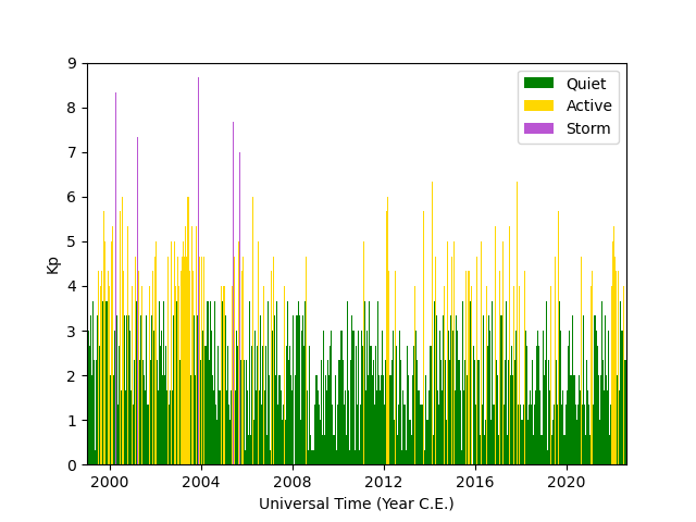
This yields 1999-01-01 00:00:00 2022-08-23 21:00:00, where the last date is your current date (not the date that I created this example). Now, we can take the combined pysat.Instrument can be used to plot the Kp over time.

fig = plt.figure()
ax = fig.add_subplot(111)

# Color code data by activity level
ax.bar(kp.data.loc[kp['Kp'] < 4, 'Kp'].index,
       kp.data.loc[kp['Kp'] < 4, 'Kp'], color='green', label='Quiet')
ax.bar(kp.data.loc[(kp['Kp'] >= 4) & (kp['Kp'] < 7), 'Kp'].index,
       kp.data.loc[(kp['Kp'] >= 4) & (kp['Kp'] < 7), 'Kp'], color='orange',
       label='Active')
ax.bar(kp.data.loc[kp['Kp'] >= 7, 'Kp'].index,
       kp.data.loc[kp['Kp'] >= 7, 'Kp'], color='firebrick', label='Storm')

# Format the figure
ax.set_xlim(stime, etime)
ax.set_ylim(0, 9)
ax.xaxis.set_major_formatter(mpl.dates.DateFormatter('%Y'))
ax.set_xlabel('Universal Time (Year C.E.)')
ax.set_ylabel(r'Kp')
ax.legend(loc=1, fontsize='medium')

# If not running in interactive mode
plt.show()

Convert Kp to ap

The Kp and ap have a well established relationship, which takes the logarithmic Kp index and converts it to a linear scale that is easier to handle numerically. The convert_3hr_kp_to_ap() converts Kp to ap, as shown below.

py_sw.instruments.methods.kp_ap.convert_3hr_kp_to_ap(kp)

print("Max: {:.1f} -> {:.1f}, Min: {:.1f} -> {:.1f}".format(
    kp['Kp'].max(), kp['3hr_ap'].max(), kp['Kp'].min(), kp['3hr_ap'].min()))

This yields Max: 9.0 -> 400.0, Min: 0.0 -> 0.0.