Make ACE SWEPAM behave like OMNI Data

NASA OMNI data (also available from pysatNASA) is the place to go for solar wind (SW) parameters. However, this data set is not available in real time. Fortunately, we can use the OMNI processing to normalize the ACE SWEPAM SW proton density and ion temperature. This is performed using the pysatSpaceWeather.instruments.methods.ace.ace_swepam_hourly_omni_norm() function. The example below uses historic ACE SWEPAM data so that we can compare the results to OMNI.

import datetime as dt
import matplotlib as mpl
import matplotlib.pyplot as plt

import pysat
import pysatSpaceWeather as py_sw
from pysatNASA.instruments import omni_hro

ace = pysat.Instrument(inst_module=py_sw.instruments.ace_swepam,
                       tag='historic', update_files=True)
omni = pysat.Instrument(inst_module=omni_hro, tag='1min', update_files=True)

# Add the OMNI conversion routine to the ACE instrument
ace.custom_attach(py_sw.instruments.methods.ace.ace_swepam_hourly_omni_norm)

# Pick a day with a geomagnetic storm
stime = dt.datetime(2014, 3, 26)

# If needed, download the data
if stime not in ace.files.files.index:
    ace.download(start=stime)

if stime not in omni.files.files.index:
    omni.download(start=stime)

# Load the data
ace.load(date=stime)
omni.load(date=stime)

print(ace.variables)

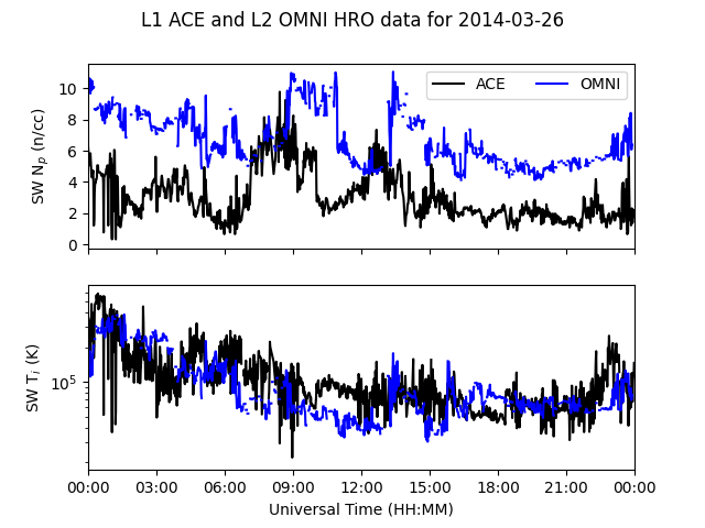
This should yield Index(['jd', 'sec', 'status', 'sw_proton_dens', 'sw_bulk_speed', 'sw_ion_temp', 'sw_proton_dens_norm', 'sw_ion_temp_norm'], dtype='object'). The variables with the 'norm' suffix were added by the conversion function. Now, let’s plot the two data sets together.

fig = plt.figure()
fig.suptitle("L1 ACE and L2 OMNI HRO data for {:}".format(stime.date()))
ax_dens = fig.add_subplot(211)
ax_temp = fig.add_subplot(212)

ax_dens.plot(ace.index, ace['sw_proton_dens_norm'], 'k-', label='ACE')
ax_dens.plot(omni.index, omni['proton_density'], 'b-', label='OMNI')
ax_temp.plot(ace.index, ace['sw_ion_temp_norm'], 'k-', label='ACE')
ax_temp.plot(omni.index, omni['T'], 'b-', label='OMNI')
ax_temp.set_yscale('log')
ax_dens.xaxis.set_major_formatter(mpl.dates.DateFormatter(''))
ax_temp.xaxis.set_major_formatter(mpl.dates.DateFormatter('%H:%M'))
ax_dens.set_xlim(stime, stime + dt.timedelta(days=1))
ax_temp.set_xlim(stime, stime + dt.timedelta(days=1))
ax_temp.set_xlabel('Universal Time (HH:MM)')
ax_dens.set_ylabel(r'SW N$_p$ ({:s})'.format(omni.meta['proton_density',
                                                       'units']))
ax_temp.set_ylabel(r'SW T$_i$ ({:s})'.format(omni.meta['T', 'units']))
ax_dens.legend(loc=1, fontsize='medium', ncol=2)

# If not running in interactive mode
plt.show()

This figure shows that the temperature adjustment agrees relatively well, but that the proton density has a large offset. This descrepency can be attributed to the data source. The pysatSpaceWeather.instruments.ace_swepam module uses L1 data, while OMNI uses L2 data that has undergone additional processing. For this time period most of the temperature data is of high quality in the L2 data, but all the proton density data is flagged for removal. The ACE L2 data is accessible through CDAWeb or the ACE database.